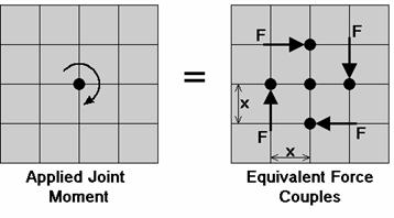
Occasionally you
may need to model an applied in-plane moment at a
This might require re-meshing the area
receiving the moment into smaller plates so that the load area can be
more accurately modeled. If a beam member is attached to the
Occasionally you
may need to model the situation where you have a beam element that is
fixed into a shear wall. A situation where this may occur would
be a concrete beam that was cast integrally with the shear wall or a steel
beam that was cast into the shear wall. The beam cannot just be
attached to the
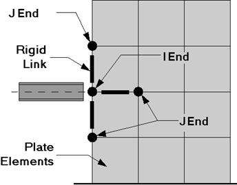
The only trick
to this method is getting the proper member end releases for the rigid
links. We want to transfer shear forces from the wall
While there is not a true “cable element”, there is a tension only element. A true cable element will include the effects of axial pre-stress as well as large deflection theory, such that the flexural stiffness of the cable will be a function of the axial force in the cable. In other words, for a true cable element the axial force will be applied to the deflected shape of the cable instead of being applied to the initial (undeflected) shape. If you try to model a cable element by just using members with very weak Iyy and Izz properties and then applying a transverse load, you will not get cable action. What will happen is that the beam elements will deflect enormously with NO increase in axial force. This is because the change in geometry due to the transverse loading will occur after all the loads are applied, so none of the load will be converted into an axial force.
You can easily model cables that are straight and effectively experience only axial loading. If the cable is not straight or experiences force other than axial force then see the next section.
When modeling guyed structures you can model the cables with a weightless material so that the transverse cable member deflections are not reported. If you do this you should place all of the cable self-weight elsewhere on the structure as a point load. If you do not do this then the cable deflections (other than the axial deflection) will be reported as very large since it is cable action that keeps a guyed cable straight. If you are interested in the deflection of the cable the calculation is a function of the length and the force and you would have to calculate this by hand.
The section set for the cable should be modeled as a tension only member so that the cable is not allowed to take compression. See T/C Members for more on this.
To prestress the cable you can apply a thermal load to create the pre-tension of the cable. See Prestressing with Thermal Loads to learn how to do this.
One way, (although not an easy one) to model a sagging cable is as follows: First you would define members with the correct area and material properties of the cable. You should use a value of 1.0 for the Iyy, Izz, and J shape properties. Next you will want to set the coordinates for your joints at a trial deflected shape for the cable. Usually you can use just one member in between concentrated joint loads. If you are trying to model the effects of cable self-weight, you will need to use at least 7 joints to obtain reasonable results. See the figure below for an example of a cable with 5 concentrated loads:
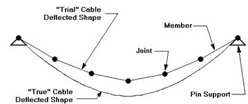
You will want to set the vertical location of each joint at the approximate location of the “final” deflected shape position. Next you will connect your members to your joints and then assign your boundary conditions. Do NOT use member end releases on your members. Make sure you do NOT use point loads, all concentrated loads should be applied as joint loads. You can model pre-stress in the cable by applying an equivalent thermal load to cause shortening of the cable.
Now you will solve the model with a P-Delta Analysis, and take note of the new vertical deflected locations of the joints. If the new location is more than a few percent from the original guess, you should move the joint to the midpoint of the trial and new location. You will need to do this for all your joints. You will repeat this procedure until the joints end up very close to the original position. If you are getting a lot of “stretch” in the cable (more than a few percent), you may not be able to accurately model the cable.
Once you are close to converging, a quick way to change all the middle joint coordinates is to use the Block Math operation. That way you shift many joints up or down by a small amount in one step.
You may model inclined supports by
using a short rigid link to span between a
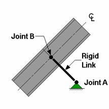
The rigid link should be “short”, say no more than 0.1 ft. The
member end releases for the rigid link at
The section forces in the rigid link
are the inclined reactions. Note that you need to make sure
the rigid link is connected to the members/plates at the correct inclined
angle. You can control the incline of the angle using the coordinates
of
The reaction at an enforced displacement can
be obtained by inserting a very short (.02' or so) rigid link between
the
Rigid links are used to rigidly
transfer the forces from one point to another and to also account for
any secondary moments that may occur due to moving the force. This
is in contrast to using the tether feature for
To Make a Rigid Link
Note
The weight density should be set to zero in case self-weight is used as a loading condition. If the material used is not weightless, then any gravity loading would cause the rigid link to add a very large load into your model. (Gravity load is applied as a distributed load with a magnitude equal to the member area times the weight density).
For models with very stiff elements, like concrete shear walls, the rigid link may not be rigid in comparison. If you see that the rigid link is deforming, then you may have to increase the stiffness of the link. The easiest way to do this is to increase the A, Iy, Iz, and J values for the RIGID section set. Make sure that the combination of E*I or E*A does not exceed 1e17 because 1e20 and 8.33e18 are the internal stiffnesses of the translational and rotational Reaction boundary conditions. If you make a member too stiff, you may get ghost reactions, which tend to pull load out of the model. (The total reactions will no longer add up to the applied loads.)
A gap element is a member that mimics the behavior of a gap or expansion joint between adjacent structures.
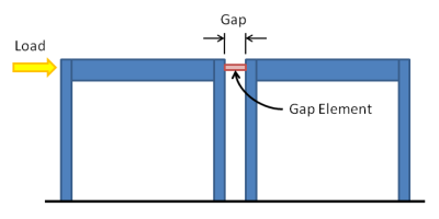
While RISA does not offer the capability to directly create a gap element, one may be indirectly created using the properties of the member and an applied thermal load. The concept is to place a ‘shrunk’ member between adjacent structures. The shrinkage of the member is achieved with a negative thermal load, in the form of a member distributed load.
The amount of shrinkage should be equal to the width of the gap, such that the structures act independently until they move close enough to each other to ‘touch’ and thereby transmit loads to each other. To calculate the thermal load required for a gap use the following formula:
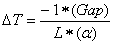
Where:
ΔT = Applied thermal load
Gap = Distance between two structures
L = Length of gap element
α = Coefficient of thermal expansion
In order to prevent the gap element from ‘pulling’ its connected structures towards it due to shrinkage it must be defined as a ‘compression only’ member under the advanced options tab. It is also advisable to define the gap element as a rigid material such that the amount of load it transfers once the gap is closed is not affected by elastic shortening.
Lastly, in cases where the applied temperature would need to be of an extraordinary magnitude, it might be useful to increase the coefficient of thermal expansion of the material such that a smaller temperature load would achieve the same shrinkage.